Three Variations on the Leaky Bucket: Queue, Meter, and Token Budget

There are three practical ways to build a rate limiter around the leaky-bucket concept. The bucket can hold requests in a queue. It can hold a running measure of recent activity. Or it can be turned upside down and expressed as a replenishing token budget.

All three combine a finite capacity with a fixed recovery rate. What changes is what the implementation stores and what happens to an accepted request: wait, pass an activity check, or spend from the available budget.

Bursts are the problem

Steady load is easy to plan for. Real traffic arrives in clumps: a scheduled job fires, a page launches forty calls, or retries land together after an outage. Network engineers describe that clumpiness with two separate limits: a sustainable rate and a burst size above it. A traffic contract needs both because an average alone says nothing about the worst second.

Capacity absorbs a bounded spike. Rate determines how quickly the system recovers. More capacity postpones overload; it never creates throughput.

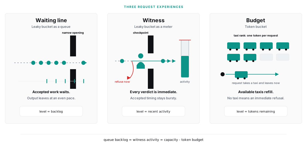
These three leaky-bucket variations put rate and capacity to work in different ways.

A waiting line

The queue is the most literal leaky bucket: a finite first-in-first-out line behind a fixed-rate opening, as described by Tanenbaum. An accepted request enters the line. Its position is both backlog and expected delay. One request leaves each service interval, so a jagged arrival pattern becomes an evenly spaced output.

The line refuses an arrival only when every waiting space is occupied. Everything already inside still leaves in order. This is traffic shaping: the mechanism changes when accepted work runs.

Nginx's limit_req follows this model when delayed requests are enabled. Its configured burst is waiting room; nodelay deliberately changes the experience by spending that room without imposing the delay.

A witness

The meter keeps the bucket but replaces stored requests with accounting. In Jonathan Turner's 1986 design, a witness keeps a gauge of recent accepted activity. Time drains the gauge. Each accepted arrival pushes it up. An arrival that would cross the limit is refused immediately and leaves the gauge unchanged.

The ITU-T standardized this idea as the generic cell rate algorithm for policing ATM traffic contracts. It is traffic policing: the mechanism changes whether work may run, not when accepted work runs. Accepted requests preserve their arrival timing, including bursts.

The gauge is memory, not storage. It records recent pressure after the accepted request has already passed the checkpoint.

A budget

The token bucket expresses the same capacity from the opposite direction. Start with a rank of available taxis. An accepted request takes one taxi and leaves immediately. Replacement taxis arrive at the refill rate. A request that finds none is refused.

The rank shows remaining opportunity rather than accumulated activity:

taxis ready = capacity - witness activity

One rises whenever the other falls. Under matched settings, witness activity and remaining budget are exact complements. Token bucket is usually presented as a separate algorithm, but its accounting is the leaky-bucket meter viewed as remaining capacity instead of accumulated activity.

Put them side by side

On larger screens, the two simulators below are independent. Each can show any of the three mechanisms without resetting its state, so you can compare any pair or give each side a different load. On mobile, one simulator provides the same three modes without squeezing the controls into a narrow comparison.

On a larger screen, start with Waiting line beside Witness and press Burst +10 on both. The admission trend matches, but the lower timelines do not: the line spaces its output while the witness passes accepted arrivals together. On mobile, run the burst in one mode, then switch modes without resetting its state.

Next compare Witness with Budget. Recent activity rises as taxis disappear, and the two levels sum to capacity. Finally, set arrivals below the configured rate on one side and above it on the other. The healthy side recovers between arrivals. The saturated side eventually refuses work regardless of its capacity.

The contrast is easiest to remember by asking what each machine stores:

• Waiting line: stores accepted requests. Its level is backlog, its output is smoothed, and a full line refuses the next arrival.
• Witness: stores recent activity. Accepted work passes immediately with its original timing, and an arrival that would cross the activity limit is refused.
• Budget: stores future admission opportunities. An accepted request spends one token and passes immediately, and an empty budget refuses the next arrival.

The shared leaky-bucket core

At their core, all three implementations track pressure against finite capacity and recover at a fixed rate. For fixed-size requests, one neutral state variable can describe that shared mechanism. Call recent admitted work L, capacity C, and the service, drain, or refill rate R:

L = max(
  0,
  L + accepted arrivals
    - R * elapsed
)

queue backlog  = L
witness activity = L
token budget   = C - L

The activity and budget forms of the admission check are complements:

accept when
  L + request cost <= C

accept when
  remaining tokens >= request cost

This is why all three are variations on the leaky-bucket concept. With matched settings, they track the same pressure and reach matching admission verdicts. The implementation policy remains different: the queue delays accepted work and controls departure timing, while the meter and token budget admit accepted work immediately.

The comparison has clear boundaries. This simulator uses fixed-size unit requests, matched capacity and rates, and the same starting state. Variable request costs, priority queues, deadlines, and other scheduling policies add behavior this state model does not contain.

From model to implementation

A production limiter can keep its accounting compact: the current level and the time it was last updated. On each arrival, subtract the recovery earned since that timestamp, test the new request against capacity, then store the result. A refusal can include the time until the next opening so the caller knows when to retry.

The queue variation needs somewhere to hold accepted work and a worker that releases it at the configured pace. The meter and budget variations need an atomic update wherever their shared state lives. In every case, capacity controls the burst and the recovery rate controls sustained throughput.

Start with the request experience you need. Choose a Waiting line to smooth accepted work, a Witness to make an immediate conformance decision, or a Budget to express the same limit as remaining burst capacity. These are three implementations of the same leaky-bucket idea: pressure accumulates against a finite capacity, time creates room again, and the policy decides what the request experiences.